Adaptive Layers
Embedding models are often encoder models with numerous layers, such as 12 (e.g. sentence-transformers/all-mpnet-base-v2) or 6 (e.g. sentence-transformers/all-MiniLM-L6-v2). To get embeddings, every single one of these layers must be traversed. The 2D Matryoshka Sentence Embeddings (2DMSE) preprint revisits this concept by proposing an approach to train embedding models that will perform well when only using a selection of all layers. This results in faster inference speeds at relatively low performance costs.
Note
The 2DMSE preprint was later updated and renamed to ESE: Espresso Sentence Embeddings. The Sentence Transformers implementation of Adaptive Layers and Matryoshka2d (Adaptive Layer + Matryoshka Embeddings) are based on the initial preprint, and we accept contributions that implement the updated ESE paper.
Use Cases
The 2DMSE paper mentions that using a few layers of a larger model trained using Adaptive Layers and Matryoshka Representation Learning can outperform a smaller model that was trained like a standard embedding model.
Results
Let’s look at the performance that we may be able to expect from an Adaptive Layer embedding model versus a regular embedding model. For this experiment, I have trained two models:
tomaarsen/mpnet-base-nli-adaptive-layer: Trained by running adaptive_layer_nli.py with microsoft/mpnet-base.
tomaarsen/mpnet-base-nli: A near identical model as the former, but using only
MultipleNegativesRankingLossrather thanAdaptiveLayerLosson top ofMultipleNegativesRankingLoss. I also use microsoft/mpnet-base as the base model.
Both of these models were trained on the AllNLI dataset, which is a concatenation of the SNLI and MultiNLI datasets. I have evaluated these models on the STSBenchmark test set using multiple different embedding dimensions. The results are plotted in the following figure:
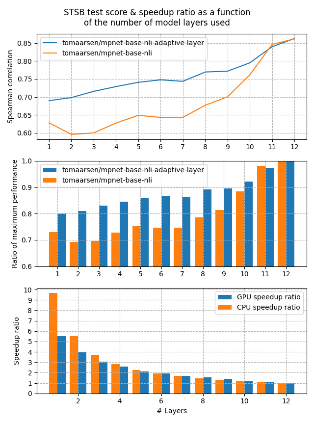
The first figure shows that the Adaptive Layer model stays much more performant when reducing the number of layers in the model. This is also clearly shown in the second figure, which displays that 80% of the performance is preserved when the number of layers is reduced all the way to 1.
Lastly, the third figure shows the expected speedup ratio for GPU & CPU devices in my tests. As you can see, removing half of the layers results in roughly a 2x speedup, at a cost of ~15% performance on STSB (~86 -> ~75 Spearman correlation). When removing even more layers, the performance benefit gets larger for CPUs, and between 5x and 10x speedups are very feasible with a 20% loss in performance.
Training
Training with Adaptive Layer support is quite elementary: rather than applying some loss function on only the last layer, we also apply that same loss function on the pooled embeddings from previous layers. Additionally, we employ a KL-divergence loss that aims to make the embeddings of the non-last layers match that of the last layer. This can be seen as a fascinating approach of knowledge distillation, but with the last layer as the teacher model and the prior layers as the student models.
For example, with the 12-layer microsoft/mpnet-base, it will now be trained such that the model produces meaningful embeddings after each of the 12 layers.
from sentence_transformers import SentenceTransformer
from sentence_transformers.sentence_transformer.losses import CoSENTLoss, AdaptiveLayerLoss

# Loading in fp32 is preferred for training if your memory can handle it
model = SentenceTransformer("microsoft/mpnet-base", model_kwargs={"torch_dtype": "float32"})

base_loss = CoSENTLoss(model=model)
loss = AdaptiveLayerLoss(model=model, loss=base_loss)
Reference:
AdaptiveLayerLoss
Note that training with AdaptiveLayerLoss is not notably slower than without using it.
Additionally, this can be combined with the MatryoshkaLoss such that the resulting model can be reduced both in the number of layers, but also in the size of the output dimensions. See also the Matryoshka Embeddings for more information on reducing output dimensions. In Sentence Transformers, the combination of these two losses is called Matryoshka2dLoss, and a shorthand is provided for simpler training.
from sentence_transformers import SentenceTransformer
from sentence_transformers.sentence_transformer.losses import CoSENTLoss, Matryoshka2dLoss

model = SentenceTransformer("microsoft/mpnet-base", model_kwargs={"torch_dtype": "float32"})

base_loss = CoSENTLoss(model=model)
loss = Matryoshka2dLoss(model=model, loss=base_loss, matryoshka_dims=[768, 512, 256, 128, 64])
Reference:
Matryoshka2dLoss
Inference
After a model has been trained using the Adaptive Layer loss, you can then truncate the model layers to your desired layer count. Note that this requires doing a bit of surgery on the model itself, and each model is structured a bit differently, so the steps are slightly different depending on the model.
First of all, we will load the model & access the underlying transformers model like so:
from sentence_transformers import SentenceTransformer

model = SentenceTransformer("tomaarsen/mpnet-base-nli-adaptive-layer")

# We can access the underlying model with `model.transformers_model`
print(model.transformers_model)
MPNetModel(
  (embeddings): MPNetEmbeddings(
    (word_embeddings): Embedding(30527, 768, padding_idx=1)
    (position_embeddings): Embedding(514, 768, padding_idx=1)
    (LayerNorm): LayerNorm((768,), eps=1e-05, elementwise_affine=True)
    (dropout): Dropout(p=0.1, inplace=False)
  )
  (encoder): MPNetEncoder(
    (layer): ModuleList(
      (0-11): 12 x MPNetLayer(
        (attention): MPNetAttention(
          (attn): MPNetSelfAttention(
            (q): Linear(in_features=768, out_features=768, bias=True)
            (k): Linear(in_features=768, out_features=768, bias=True)
            (v): Linear(in_features=768, out_features=768, bias=True)
            (o): Linear(in_features=768, out_features=768, bias=True)
            (dropout): Dropout(p=0.1, inplace=False)
          )
          (LayerNorm): LayerNorm((768,), eps=1e-05, elementwise_affine=True)
          (dropout): Dropout(p=0.1, inplace=False)
        )
        (intermediate): MPNetIntermediate(
          (dense): Linear(in_features=768, out_features=3072, bias=True)
          (intermediate_act_fn): GELUActivation()
        )
        (output): MPNetOutput(
          (dense): Linear(in_features=3072, out_features=768, bias=True)
          (LayerNorm): LayerNorm((768,), eps=1e-05, elementwise_affine=True)
          (dropout): Dropout(p=0.1, inplace=False)
        )
      )
    )
    (relative_attention_bias): Embedding(32, 12)
  )
  (pooler): MPNetPooler(
    (dense): Linear(in_features=768, out_features=768, bias=True)
    (activation): Tanh()
  )
)
This output will differ depending on the model. We will look for the repeated layers in the encoder. For this MPNet model, this is stored under model.transformers_model.encoder.layer. Then we can slice the model to only keep the first few layers to speed up the model:
new_num_layers = 3
model.transformers_model.encoder.layer = model.transformers_model.encoder.layer[:new_num_layers]
Then we can run inference with it using SentenceTransformers.encode.
from sentence_transformers import SentenceTransformer

model = SentenceTransformer("tomaarsen/mpnet-base-nli-adaptive-layer")
new_num_layers = 3
model.transformers_model.encoder.layer = model.transformers_model.encoder.layer[:new_num_layers]

embeddings = model.encode(
    [
        "The weather is so nice!",
        "It's so sunny outside!",
        "He drove to the stadium.",
    ]
)
# Similarity of the first sentence with the other two
similarities = model.similarity(embeddings[0], embeddings[1:])
# => tensor([[0.7761, 0.1655]])
# compared to tensor([[ 0.7547, -0.0162]]) for the full model
As you can see, the similarity between the related sentences is much higher than the unrelated sentence, despite only using 3 layers. Feel free to copy this script locally, modify the new_num_layers, and observe the difference in similarities.
Code Examples
See the following scripts as examples of how to apply the AdaptiveLayerLoss in practice:
adaptive_layer_nli.py: This example uses the
MultipleNegativesRankingLosswithAdaptiveLayerLossto train a strong embedding model using Natural Language Inference (NLI) data. It is an adaptation of the NLI documentation.adaptive_layer_sts.py: This example uses the CoSENTLoss with AdaptiveLayerLoss to train an embedding model on the training set of the STSBenchmark dataset. It is an adaptation of the STS documentation.
And the following scripts to see how to apply Matryoshka2dLoss:
2d_matryoshka_nli.py: This example uses the
MultipleNegativesRankingLosswithMatryoshka2dLossto train a strong embedding model using Natural Language Inference (NLI) data. It is an adaptation of the NLI documentation.2d_matryoshka_sts.py: This example uses the
CoSENTLosswithMatryoshka2dLossto train an embedding model on the training set of the STSBenchmark dataset. It is an adaptation of the STS documentation.